Parameters and growth model of the bimTree

Introduction

The parameters ofor the form and the growth curved are based on extensive data analysis combined with tree nursery stock information. The later ones are the starting point of our simulation (size at planting time) and the growth curve descripes the transition over time towards the fianal form and size.

The Cescatti-Hull-Model

We adapted the asymmetric hull model originally proposed by Horn [13] and Koop [14] and then extended by Cescatti [15]. The envelope is defined using six control points and two shape factors. By connecting the four Point (p1 to P4) with four elliptical quarters in XY-plane and interpolated height (Z) the peripheral line L is defined. The Line separates the crown in to the upper (light) and lower (shadow) part. Points on the Line L are connected to the top and bottom point (PT, PB) by super-ellipses with degree cT and cB. This two parameters control the curvature of the super-ellipses and we assume that CT and CB are constant for all parts of the crown. The tangents at the endpoints of the ellipse are perpendicular (for concave forms) or parallel (for convex forms ) to the XY-Plane to create transitions between the lower and upper part. With a few easily controllable parameters, a large variety of realistic crown shapes can be archived, We will use the model to represent asymmetric existing trees

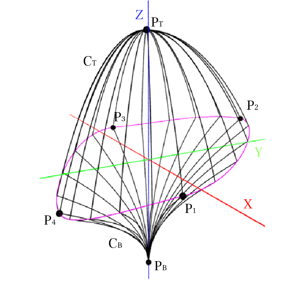
The Simplified Cescatti-hull-Model for symmetric trees and root representation

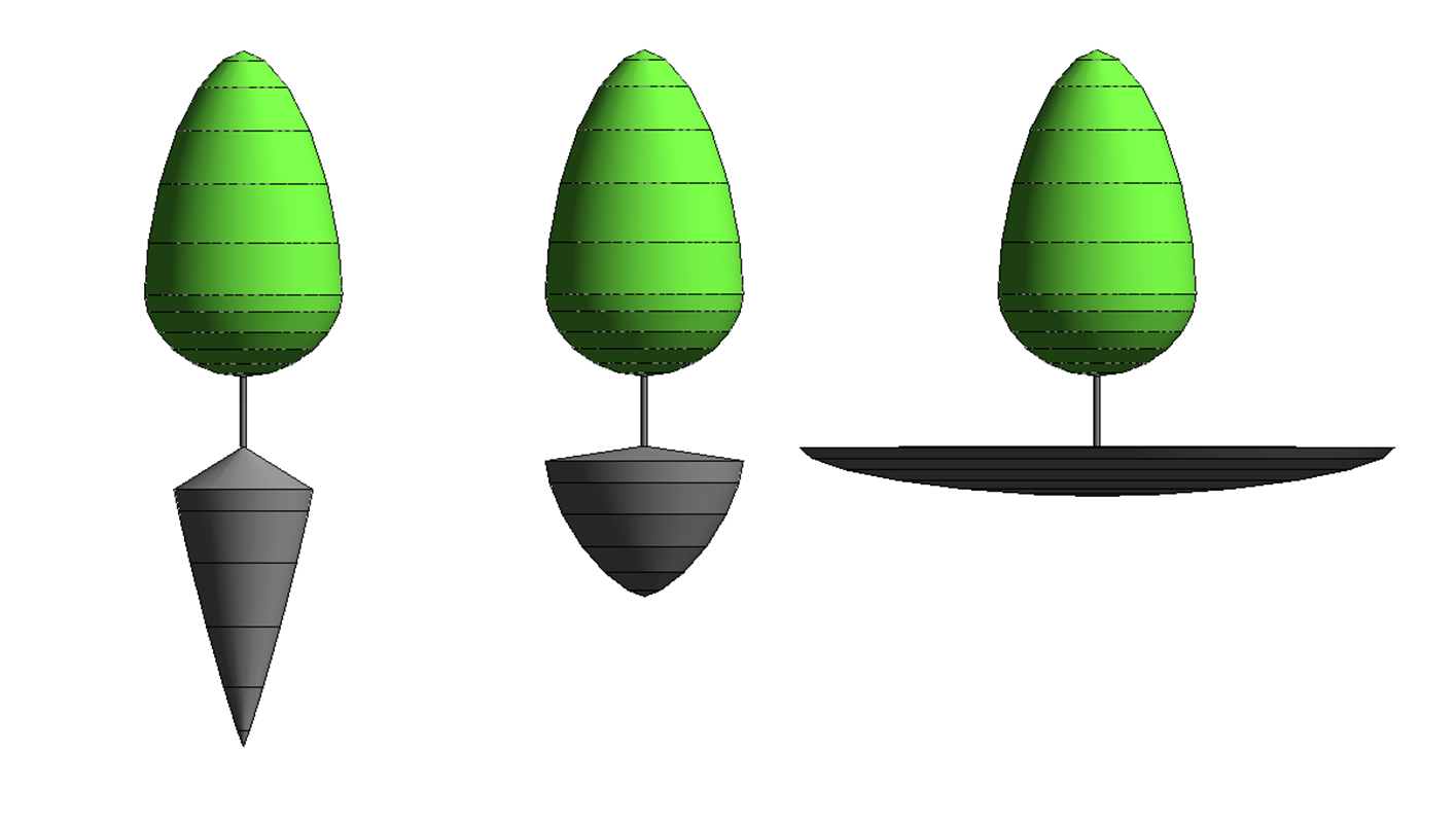
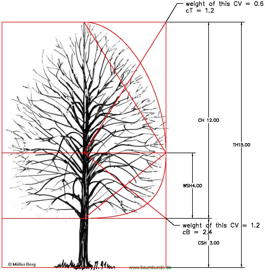
For symmetric trees the model can be simplified and aligned with commonly used specification of nursery stocks. The Points P1 to P4 are on a circle all at the Height of the Largest Crown Radius.

Points	x	y	z
PB	Insert point	Insert point	Height Clear Stem
PT	Insert point	Insert point	Height Tree
P1, P3	Insert Point +/- Tree Spread/ 2	Insert Point	Height Largest Crown Radius
P2, P4	Insert Point	Insert Point +/- Tree Spread/ 2	Height Largest Crown Radius

Table 1: Form parameters and Cescatti-hull points

We adapted a modified version of the model to create the root envelope based on relations between crown radius and radius and depth of the root in for typical root forms.

Chapman-Richards Growth Model

There is a wide range of growth functions. We selected the Chapman-Richards model (Richards, 1959). as this function has been one of the most popular model for describing the growth of various trees with forest stand growth variables, e.g. tree and stand height, diameter at breast height, basal area and volume. It has been widely used in many empirical forest growth simulators, particularly when the accuracy of model prediction is crucial (Tjørve and Tjørve, 2010).. In the Richard-Chapmann form, the curve starts with germination and has therefore only three parameter. Its most compact form is as follows:

h(t) = hmax * (1- exp(-k*t))^p

It produces sigmoid shapes for p>1, where h_max is the maximum height (upper limit). The parameters k and p have no direct meaning, but

ti = ln (p)/k;
h(ti) = hmax * (1-1/p) ^p;
K = hmax * k *((p-1)/p)^(p-1) 

where t_i is the time of the fastest growth h(t_i) is the size at this time and K is the maximum growth rate, values for direct interpretation of important characteristics of observed growth patterns with meaningful interpretation (Tjørve and Tjørve, 2010).

Determination of form parameters

The parameters for the super-ellipses that describing the shape of the tree we can find by simple tracing images (silhouettes) of this trees with super-ellipses in CAD or adapting values from similar trees.

Determination of growth models

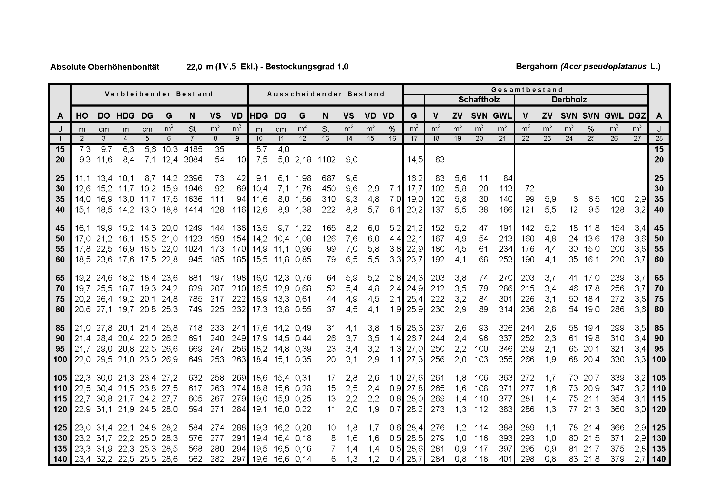
In the first step we review literature to find existing equations, we may can transform to Chapman-Richards-models or using statistical analysis (robust regression) to evaluate existing growth data like forest growth and stand information (black dots and lines)

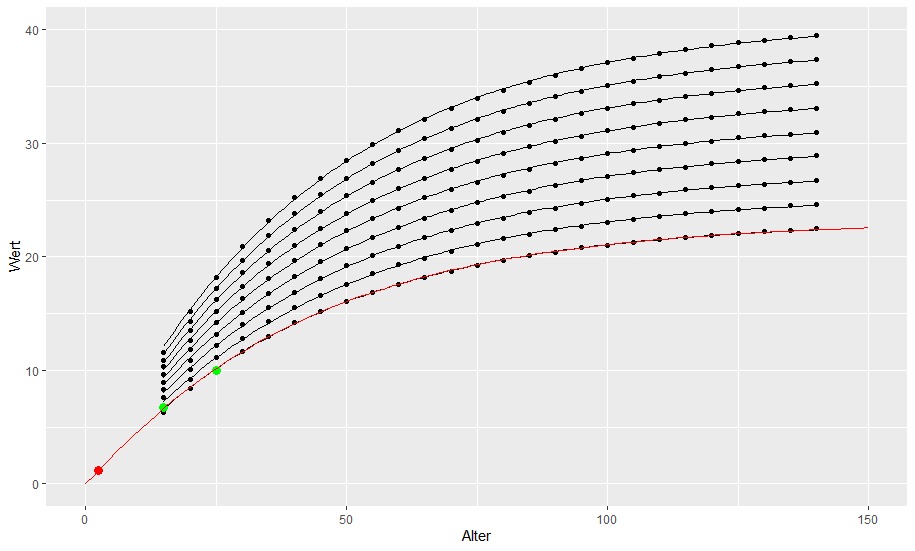
As the graphic show, the shape of the curves (described by the p and k value) are consistent in different stands, only the upper asymptote or final value varies.

We selecting the curve (red line) thats aligns with known heights in landscape/urban settings and known maximum values.

We also reviewing the point of fastest growth (inflection point, red) and the growth rate in this point with (45 cm/year in the second year) for plausibility as well as with tree nursery stock specifications and expected final size. Therefore we allow in our simulation software the adjustment of the final size based on site conditions (site index).

Start values

The simulation starts with the size defined by the tree nursery specification and a calculated relative growth to address the that trees from nurseries may differ from the forest counterparts. Over time the curve based on relative growth is approximating the growth curve based on absolute growth and is in mature age the difference is insignificant.

The resulting curve has an almost identical form, even the parameters showing notable differences. This form of the model restricts values for d to 0 < d < 1 and subsequently the value for DBH(T_i) < A/e.

---

Citations:

Richards, F. J. (1959). "A Flexible Growth Function for Empirical Use". Journal of Experimental Botany. 10 (2): 290–300. doi:10.1093/jxb/10.2.290.

Tjørve E, Tjørve KM. (2010). A unified approach to the Richards-model family for use in growth analyses: why we need only two model forms. J Theor Biol. 2010 Dec 7;267(3):417-25. doi: 10.1016/j.jtbi.2010.09.008. Epub 2010 Sep 8. PMID: 20831877.